AWS Foundational Skills: Optimizing AWS costs with the Cost and Usage Report (CUR)

Welcome back to our Foundation series, in which we take a deep dive into the tools and services that make up – you guessed it – the foundation of a successful FinOps practice and AWS cost optimization initiative. 

We started with CloudWatch and Systems Manager, which we referred to as the brain and nervous system of AWS respectively. Continuing that analogy, today’s topic, the Cost and Usage Report (CUR), would be the metabolic system. It’s where the energy that goes into the system (money) is turned into all of the low-level activities that power the system as a whole.

To set the stage for the importance of the Cost and Usage Report, please indulge me in revisiting a classic sci-fi movie, Star Trek II, the Wrath of Khan. Towards the end of the movie, Captain Kirk, Lieutenant Spock, and the crew of the Enterprise find themselves backed into a corner by Khan, their nemesis. Khan is powerful, smart, focusing his wrath on the Enterprise and her crew, and trying to steal scientific research from the data banks of the Enterprise to repurpose into a destructive weapon.

Khan has the upper hand in all ways but one. Kirk and Spock have the low-level data, the understanding of “how things really work aboard a starship.” With this knowledge, they’re able to remotely disarm the Khan’s shields and win the day!

The Cost and Usage Report is “how things really work” in an AWS account, at least in terms of cost. It’s the low-level data of every service that can incur a charge. It is this data that can inform us about the structure of AWS accounts and help us understand exactly where the spend occurs.

In this guide, we’re going to talk about what the Cost and Usage Report is, how to set it up and query it, and most importantly, how to truly understand your AWS spend at an organizational level.

Table of contents

1. A brief overview of AWS Cost and Usage Reports
2. How the Cost and Usage Report is structured and used
3. Setting up AWS Cost and Usage Reports
4. Using AWS Athena to query the CUR
   1. Querying the CUR: NAT Gateways
   2. Querying the CUR: Exploring Neptune costs
   3. Querying the CUR: EC2 usage
   4. How we use the CUR in CloudFix finder/fixers
5. A few final notes on the CUR
   1. Blended vs. unblended costs
   2. Savings Plans
   3. Cloud Intelligence Dashboards
6. Go forth and save!

1. A brief overview of AWS Cost and Usage Reports

The AWS Cost and Usage Report is described in the official documentation as “the most comprehensive set of cost and usage data available.” Commonly known as the CUR (pronounced “curr”, rhyming with “purr”), it gives you cost data broken down by hour, day, or month for every AWS service. The indispensable feature of the CUR is that it works at the master payer account level. It gives us a complete overview of spend not just in an account, but across an entire organization.

The CUR is used by nearly all CloudFix finder/fixers to identify resources within an organization. Additionally, due to the usage-based pricing of most resources, we also use the CUR data to understand how resources are being used. For example, resources such as VPC endpoints are priced both per hour and per usage. If the CUR data contains only the hourly portion but not the metered, usage-based portion, then we know that this resource is not being utilized.

For other resources, we can use the CUR to gain a list of all assets in an account, and then use CloudWatch to determine idleness. This is the approach we take with, for example, idle Neptune clusters: a CUR query finds the database instances and CloudWatch determines if the clusters are idle or not.

Finally, the CUR powers the Cloud Intelligence Dashboards. These dashboards, built by AWS Technical Account Managers, have been tailored to help AWS clients understand and control their spend. Watch these clips from AWS Made Easy, where Rahul and I talk with AWS guests about the power of these dashboards.

2. How the Cost and Usage Report is structured and used

At its heart, the CUR can be thought of as an hourly itemized receipt for all AWS spend. It is a large table, generated daily, where each row represents allocation of spend to a particular item. If you added the cost across every single row for an entire month, it would be equal to your AWS bill. In other words, the CUR lets you see how every penny of your AWS spend is allocated.

Operationally, the reports are generated on a daily basis and placed in a specified S3 bucket (more on this below). The data in the S3 buckets is provided in CSV format and cannot be directly queried. Luckily, AWS has a fantastic service, AWS Athena, that can ingest CSV files in an S3 bucket and provide a SQL interface for querying these files. 

When we use the term “CUR query”, what we’re really saying is that we are using Athena to query the CSV files that collectively comprise the Cost and Usage Report. As we configured in the previous section, these CSV files get generated and added to a specified S3 bucket on a daily basis.

The types of data returned by the CUR are divided into:

1. Identity details
2. Billing details
3. Line item details
4. Reservation details
5. Pricing details
6. Product details
7. Resource tags details
8. Savings plans details
9. Cost categories details
10. Discount details
11. Split line item details

A full explanation of the data category is available in the comprehensive Data Dictionary. There are an infinite number of ways to query, join, and aggregate this data. We’re going to focus on resource usage queries, where we are looking at the amount of usage of a particular resource over time. The columns that tend to feature highly in these queries are:

• product/Region – The region where the resources exist.
• lineItem/UsageAccountId – The account that created/consumed the resource.
• lineItem/ResourceId – This is almost always an ARN, like of an EC2 instance, DynamoDB table, etc.
• lineItem/LineItemType – The type of charge being accounted for in this row. We often filter this to look for type of Usage, meaning the on-demand or metered cost. Other values for this field include Tax and charges related to savings plans.
• lineItem/UsageStartDate, lineItem/UsageEndDate – The start and end dates for the usage in question.
• lineItem/UsageType – These are details about the usage. For example, for VPC NAT Gateways, values of this column may be NatGateway-Bytes and NatGateway-Hours, as NAT gateways charge both a per-hour fee and a per-byte fee.
• lineItem/UnblendedCost – The cost for the particular line item. We will talk about the “unblended” term later in the article.

Next, let’s have a look at setting up a CUR for your organization.

3. Setting up AWS Cost and Usage Reports

In this section, we’re going to review the main steps for setting up your own Cost and Usage. For a comprehensive guide, follow the excellent Well Architected Labs by AWS.

At a high level, in order to set up a Cost and Usage Report:

1. Log into your Management Console using the master payer account. Go to the Billing console and select Cost and Usage Reports.
2. You need to enter a report name and S3 bucket name. AWS recommends that the account number be part of the CUR report name, e.g. “###########-CUR” where ########### is your management account number.
3. Check the settings:
   1. Output to a valid S3 bucket with reasonable prefix
   2. Time Granularity is set to Hourly
   3. Report additional content: Include resource IDs
   4. Report Versioning: We recommend having the reports accumulate, rather than replace the existing version.
   5. Enable report data integration for Amazon Athena, in parquet format.
4.  If the settings are correct, click “Review and Complete”.

Now that the CUR is set up, we need to set up Athena. This will allow us to query the report data using SQL. To set up Amazon Athena, you should follow the Querying Cost and Usage Reports using Amazon Athena guide. As a quick overview:

1. The CUR includes a CloudFormation template for setting up an Athena stack. Download it from S3.
2. Open the CloudFormation console, choose Create New Stack, and then Create Stack.
3. Upload the template .yml file you just downloaded.
4. Approve the creation of the resources proposed: 3x IAM roles, an AWS Glue database, an AWS Glue Crawler, two Lambda functions, and an S3 notification.

Once the stack has been created successfully, you can run SQL queries using Amazon Athena. The easiest way to get started is to use the web interface.

4. Using AWS Athena to query the CUR

As we mentioned earlier, we don’t query the CUR directly. Instead, we use AWS Athena, which provides a SQL interface to the large collection of CSV files that collectively are your CUR.

Athena can be accessed in several different ways:

1. Athena web console: The easiest way to get started. It provides a visual query interface, is simple to use, and offers syntax and autocompletion.
2. Using an AWS SDK, such as boto3: This may be the most robust option, as it can be embedded into automated processes.
3. Using ODBC: This approach uses the standard SQL connectivity protocol, ODBC, to connect to the database. This is best for integration with visualization and analytics tools.

The most important thing is that you get the data out and start crunching the numbers! If you’re new to Athena, go check out the Getting started with Amazon Athena document. In the rest of this section, we develop sample queries for 3 different topics: NAT Gateways, Amazon Neptune, and EC2.

4.1. Querying the CUR: NAT Gateways

Let’s do a simple query looking for NAT gateways. This is the query we use for the idle VPC Nat Gateway finder/fixer. The query of interest is the following:

SELECT product_region,
        line_item_usage_account_id,
        line_item_resource_id,
        line_item_line_item_type,
        line_item_usage_start_date, 
        line_item_usage_end_date, 
        line_item_usage_type,
        sum(line_item_unblended_cost) as cost
 FROM "YOUR_CUR_DB_NAME"."YOUR_CUR_TABLE_NAME" 
 WHERE line_item_line_item_type = 'Usage' 
   AND line_item_usage_start_date >= date_trunc('day', current_date - interval '31' DAY) 
   AND line_item_usage_start_date < date_trunc('day', current_date - interval '1' DAY) 
   AND (line_item_usage_type LIKE '%NatGateway-Hours%' OR line_item_usage_type LIKE '%NatGateway-Bytes%')
GROUP BY 1,2,3,4,5,6,7;

Let’s look at each clause of this query one at a time. The SELECT statement is asking for the set of columns mentioned in the previous section. Note that we convert the data dictionary column name format (category/ColumnCamelCase) into snake_case. We need to do this, as SQL column names are not case sensitive and cannot contain the / character. The only aggregation we’re doing is a sum operator over the cost.

The FROM clause needs to be modified to reference your CUR database and CUR table name that was configured when you configured your organization’s CUR. Looking at the WHERE clauses, we are filtering on line_item_line_item_type by Usage. This includes both hourly charges and data-based charges: NAT Gateways have both! We are also filtering by line_item_usage_start_date and line_item_usage_end_date. Our CUR is set up for hourly reporting, so for a given row in the data set line_item_usage_end_date will be exactly one hour later than line_item_usage_start_date. This means that the charges accounted for by this row take place during the hour specified. 

Finally, we are looking for line-item-usage-type matching two different expressions, NatGateway-Hours or NatGateway-Bytes. These are the two different types of usage charges we can get using NAT gateways. The data from this query looks like the following:

Analyzing the sample data, note that the resources returned span multiple account regions and accounts. This is because we are looking at a master payer account, which has many accounts within it. For brevity, the account numbers have been shortened; they are typically 12 digits. As expected, the span between the line_item_usage_start_date and line_item_usage_end_date is one hour. 

Notice the line_item_usage_type that matches our regular expressions %NatGateway-Hours% and NatGateway-Bytes. These are the two ways in which NAT gateways incur usage-based charges. Some entries in this column have prefixes corresponding to the region in which they exist. For example, APS2-NateGateway-Hours charges are incurred for NAT gateways located in the ap-southeast-2 region.

A few thoughts for this example:

1. This query demonstrates how to list resources across accounts and regions without needing to manage many different sets of permissions or make API calls. This was all done in one query!
2. We have detailed data, down to the hour, about the types of charges each resource was incurring. We can use SQL constructs such as SORT to find the most expensive resources.
3. The resources are identified by their Amazon Resource Name (ARN). This is almost always the case, but there are some exceptions, most notably EC2.
4. There is information communicated both by the presence and absence of data. In this case, we know that all NAT gateways incur an hourly charge, but only NAT gateways that are moving data incur a -Bytes charge. This allows us to build higher order logic using SQL joins. For insance, we could use one query to collect all ARNs and then use a LEFT JOIN to find NAT gateways that do not have NatGateway-Bytes charges.

4.2 Querying the CUR: Exploring Neptune costs

Neptune, Amazon’s Graph Database offering, is relatively new on the scene. It’s powered by RDS, and the pricing model for Neptune is based on RDS instance usage as well as data storage and IO. In a large organization, there are likely to be many teams who have tried Neptune, and we want to make sure that there are no idle Neptune clusters racking up charges. At CloudfFix, we have a finder/fixer that does exactly that. 

As part of exploring what Neptune-related data is available within the CUR, it can be useful to look at the values for line_item_usage_type for a particular service. We can do this with the distinct SQL command. Here is an example of doing that with Neptune:

SELECT DISTINCT line_item_usage_type
FROM "YOUR_CUR_DB_NAME"."YOUR_CUR_TABLE_NAME" 
 WHERE
    line_item_product_code = 'AmazonNeptune'
    AND line_item_usage_start_date >= date_trunc('day', current_date - interval '31' day)
    AND line_item_usage_start_date < date_trunc('day', current_date - interval '1' day)
ORDER BY line_item_usage_type;

In one account we scanned (which represents typical usage), I saw the following result:

This small data set already tells a story. From this query, we can learn that:

• This organization is using both Neptune Serverless and standard Neptune, which is backed by RDS instances. In our idle Neptune finder/fixer blog post, we note that compute instances for Neptune look like RDS instances, as they are backed by RDS.
• Neptune is being used in both us-east-1 and us-west-2. We can tell this because BackupUsage has no prefix, so we can assume us-east-1. The final entry, USW2-BackupUsage, indicates that there are also Neptune charges for backups in us-west-2.
• This organization is using three different instance types for Neptune. Of these types, two are Graviton-based, the r6g.xl and the t4g.medium. The other type is the value-based t3.medium instance.
• Finally, note that the first row, being blank, is not a mistake. There are some rows where this does not apply. This typically happens when the LineItemType is Tax.

Now that we have a bit of understanding about the account, perhaps we are interested in all of the (account, region) pairs across the organization where Neptune is being used. To do this, we could run the following query:

SELECT DISTINCT product_region, line_item_usage_account_id 
FROM "YOUR_CUR_DB_NAME"."YOUR_CUR_TABLE_NAME" 
WHERE
   line_item_product_code = 'AmazonNeptune'
   AND line_item_usage_start_date >= date_trunc('day', current_date - interval '31' day)
   AND line_item_usage_start_date < date_trunc('day', current_date - interval '1' day)

This query would return two columns, with each row containing a region/account pair where Neptune has been used within the past 31 days. For example, the output may look like:

Or maybe you’re interested in clusters that have incurred some IO usage in the past 31 days. To do this, we can filter on the line_item_resource_id to look for :cluster: inside the ARN. To do this in SQL, we could use the following query:

SELECT
    product_region,
    line_item_usage_account_id,
    line_item_resource_id,
    line_item_line_item_type,
    line_item_usage_type,
    sum(line_item_unblended_cost) as cost
 FROM "YOUR_CUR_DB_NAME"."YOUR_CUR_TABLE_NAME"
 WHERE
    line_item_product_code = 'AmazonNeptune'
    AND line_item_usage_start_date >= date_trunc('day', current_date - interval '31' day)
    AND line_item_usage_start_date < date_trunc('day', current_date - interval '1' day)
    AND line_item_resource_id like '%:cluster:%'
 GROUP BY 1,2,3,4,5
 ORDER BY cost desc;

A key observation here is that we’re using a regular expression on the resource_id. Running this query, we would have results like the following:

Looking over the data, we may notice that line_item_usage_type is either StorageIOUsage, BackupUsage, or StorageUsage. There are no instance-based charges for the nodes in this cluster here. This is because the nodes of the cluster are billed against the node resource, rather than the cluster resource. To look at the individual instances, we can modify the line_item_resource_id to match “arn:aws:rds:“.

The query would look like:

SELECT
   product_region,
   line_item_usage_account_id,
   line_item_resource_id,
   line_item_line_item_type,
   line_item_usage_type,
   sum(line_item_unblended_cost) as cost
FROM "YOUR_CUR_DB_NAME"."YOUR_CUR_TABLE_NAME" 
WHERE
   line_item_product_code = 'AmazonNeptune'
   AND line_item_usage_start_date >= date_trunc('day', current_date - interval '31' day)
   AND line_item_usage_start_date < date_trunc('day', current_date - interval '1' day)
   AND line_item_resource_id like '%arn:aws:rds%'
GROUP BY 1,2,3,4,5
ORDER BY cost desc;

and the sample data would look like: 

Note that the ARNs are now RDS instances, since as we mentioned, Neptune clusters are based on RDS instances. Finally, note that there is not a way to determine the association between a cluster and an ARN using the CUR. To do this, we need to describe each Neptune instance with the aws neptune describe-db-instances command. This illustrates an important point: the CUR does not contain configuration data. In order to get a full picture of the configuration, you can supplement CUR data with data from the other AWS APIs.

The takeaways here:

• You can use regular expressions with the SQL like command to match on particular ARNs. Resources of different types have different formats of ARNs. This ARN cheat sheet can be useful. BONUS: If you are clever with SQL, you can not just match ARNs, but actually extract the components into their own columns.
• Different resource types can have different values for the line_item_usage_type field. Neptune clusters are associated with StorageIOUsage, BackupUsage, and StorageUsage. Neptune instances are associated with InstanceUsage:db.XXX.YYY where XXX is the instance type and YYY is the size, e.g. r6g.xl.
• Use the distinct keyword to explore the data for a particular product. Validate this with your own knowledge of how the product is billed.
• Not all data is contained within the CUR, especially data about associations between resources. To get this data, you can use the associated APIs. These are usually prefixed by a describe-. In this example, we use Neptune’s describe-db-instances to find the cluster associated with a particular DB instance.

4.3 Querying the CUR: EC2 usage

Now let’s talk using the CUR for EC2, which includes a few interesting caveats. The first is that AWS instances are not given an ARN. Therefore, we can’t filter on line_item_resource_id the way we had previously.

However, this is not as limiting as it would appear, as there are several ways to query for EC2 instances. Let’s have a look at an exploratory query that will list EC2 instances that have incurred charges within the last 31 days.

   SELECT product_region,
	  line_item_usage_account_id,
	  line_item_resource_id,
	  line_item_line_item_type,
	  line_item_usage_start_date, 
	  line_item_usage_end_date, 
	  line_item_usage_type, 
	  sum(line_item_unblended_cost) as cost
   FROM "YOUR_CUR_DB_NAME"."YOUR_CUR_TABLE_NAME"
   WHERE line_item_resource_id LIKE 'i-%'
     AND line_item_usage_start_date >= date_trunc('day', current_date - interval '10' DAY) 
     AND line_item_usage_start_date < date_trunc('day', current_date - interval '1' DAY) 
      GROUP BY 1,2,3,4,5,6,7;

In the above query, we are matching resource IDs to items that look like EC2 instances. Note that we do not have a leading % character in the match line, WHERE line_item_resource_id LIKE 'i-%' This matches EC2 instance identifiers. Let’s have a look at some sample data from the query.

Take note of a few features here. There are different combinations of line_item_type and usage_type. We see that there are some instances of DiscountedUsage. This is due to savings plans. Also note that the usage_type contains data transfer in and out of the region.

Let’s focus on demand instance usage that is not covered by savings plans. To do this, we can add constraints to look for Usage line_item_type and BoxUsage to the usage type. Let’s also remove the start and end times, so we can get a 31 day aggregation. Finally, we add a clause to look for only those instances where cost > 0.

SELECT product_region,
	  line_item_usage_account_id,
	  line_item_resource_id,
	  line_item_line_item_type,
	  line_item_usage_type, 
	  sum(line_item_unblended_cost) as cost,
	  product_instance_type
FROM "YOUR_CUR_DB_NAME"."YOUR_CUR_TABLE_NAME"
WHERE line_item_resource_id LIKE 'i-%'
     AND line_item_usage_start_date >= date_trunc('day', current_date - interval '10' DAY) 
     AND line_item_usage_start_date < date_trunc('day', current_date - interval '1' DAY) 
     AND line_item_line_item_type LIKE 'Usage'
     AND line_item_usage_type LIKE '%BoxUsage%'
GROUP BY 1,2,3,4,5
HAVING sum(line_item_unblended_cost) > 0; 

Note that we have also created an instance_type column that has been extracted from the usage type. Also note the use of the HAVING keyword: Athena uses the Presto SQL query engine and syntax.

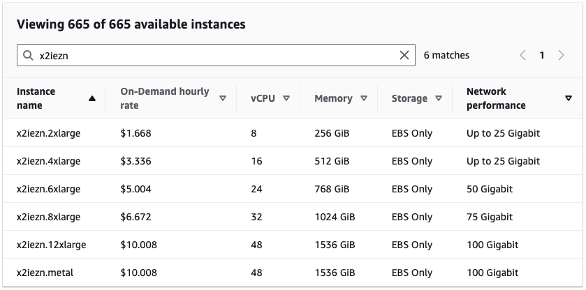
This may serve as the source of a cost alerting dashboard. For example, the x2iezn instance types are quite expensive, as seen in the screenshot of the EC2 instance pricing site. It could be good to build a dashboard from here that creates a leaderboard of expensive instance types. It may be worthwhile to be spending $10.008 per hour, but you probably want to keep tabs on this.

Finally, we’ll create a report on spot instance usage, broken down by instance type. To do this, we can wrap the above query in a subquery that groups by instance_type and aggregates total_cost.

SELECT product_instance_type, 
       SUM(cost) as total_cost 
FROM (       
SELECT product_region,
	  line_item_usage_account_id,
	  line_item_resource_id,
	  line_item_line_item_type,
	  line_item_usage_type, 
	  sum(line_item_unblended_cost) as cost,
	  product_instance_type
FROM "YOUR_CUR_DB_NAME"."YOUR_CUR_TABLE_NAME"
WHERE line_item_resource_id LIKE 'i-%'
     AND line_item_usage_start_date >= date_trunc('day', current_date - interval '10' DAY) 
     AND line_item_usage_start_date < date_trunc('day', current_date - interval '1' DAY) 
     AND line_item_line_item_type LIKE 'Usage'
     AND line_item_usage_type LIKE '%SpotUsage%'
GROUP BY 1,2,3,4,5
HAVING sum(line_item_unblended_cost) > 0
) subquery_table GROUP BY product_instance_type order by total_cost desc;

Data from this query may look like:

We can also do this analysis by product_instance_type_family:

Looking at this table, we see that the heaviest usage of spot, sorted by cost, are the t3 instance in various sizes and the m5 instance type. Using this information, we may want to ask the users of spot instances to consider retyping their spot code to the T4g Graviton instance type and the users of M5 to possibly consider M6a, M6g, M7a, or M7g instance types, which may offer better price/performance. 

When using spot instances, be sure to read the Allocation Strategies for Spot Instances document and plan accordingly. With spot, there is a tradeoff to be made in terms of price vs. efficiency. At on-demand rates, for a computationally intensive job we would always prefer a M7g over an M6g, but with spot the price/performance calculation changes. This is a subject for another day, but the key point here is that we can get a high-level overview of the general usage patterns of EC2 across an organization.

To wrap this up:

• To find EC2 instances in the CUR, you can match on the distinct ‘i-abc123’ EC2 identifier pattern.
• There are several charges associated with EC2. These include BoxUsage for on demand, SpotUsage for spot, and other charges for data transfer. You can drill down on particular charge types by filtering on line_item_usage_type.
• The product_instance_type and product_instance_type_family codes give us details about the EC2 instance.
• Take advantage of SQL aggregation and subqueries to build reports, dashboards, and leaderboards to highlight top spend in various categories. This can be used to highlight areas where improvements can be made, like the spot instance allocation strategy.

4.4. How we use the CUR in CloudFix finder/fixers

The CUR plays a critical role in CloudFix’s ability to identify and implement AWS savings opportunities. Here’s how some of our top fixers use the CUR to power AWS cost optimization. 

5. A few final notes on the CUR

While the following topics aren’t central to using the CUR, they are important parts of AWS cost optimization and important to think about and understand. 

5.1. Blended vs. unblended costs

You may see the term line_item_unblended_cost in the queries. From the many Will it Blend videos produced by Tom Dickson, CEO of the Blendtec corporation, we know that if something is blended, it must have been unblended at some point.

In Cost and Usage Report context, blended refers to AWS Reserved Instance pricing. The main idea behind blended costs is that in AWS organizations with consolidated billing and which use reserved instances, the blended cost is the average cost between the Reserved Instance usage and the on-demand usage, weighted by actual usage. Blended costs tend to be cheaper than unblended costs because they are averaging in Reserved Instance pricing, which has a lower effective hourly cost.

For the purposes of this document, where the CUR queries are being used to determine usage, we utilize the unblended cost. It is important to be aware of Reserved Instances in general. Note that, according to AWS’s own documentation on Reserved Instances, Savings Plans are recommended over Reserved Instances. Which brings us too…

5.2. Savings Plans

Savings Plans, according to AWS, are “a flexible pricing model that can help you reduce your bill by up to 72% compared to On-Demand prices, in exchange for a one- or three-year hourly spend commitment.” Savings Plans that involve EC2 are either Compute Savings Plans or EC2 Instance Savings Plans. The former is more flexible and exchanges a commitment to use a certain amount of EC2 for a cost reduction of up to 66%. The latter offers more savings, but the commitment is to a particular instance family, and region. This allows AWS to have more certainty about usage, and thus offer steeper discounts.

The Cost and Usage Report offers detailed information about Savings Plan usage, terms, and other information. There are several values of lineItem/LineItemType relating to savings plans. They all begin with savings_plan_.

You can even track your usage relative to committed spend. From the Cost and Usage Report – Understanding Savings Plans documentation:

5.3. Cloud Intelligence Dashboards

The Cost and Usage Report also powers a family of dashboards called the Cloud Intelligence Dashboards. One of these dashboards is called the Cost and Usage Dashboards Operations Solutions, commonly called the CUDOS dashboard. The CUDOS dashboard provides comprehensive cost and usage details at an organization level, but with resource-level granularity. With the CUDOS dashboard, you can look at spend per AWS product, broken down by month. You can visualize the month-over-month changes in spend, perform an analysis per region, and much more.

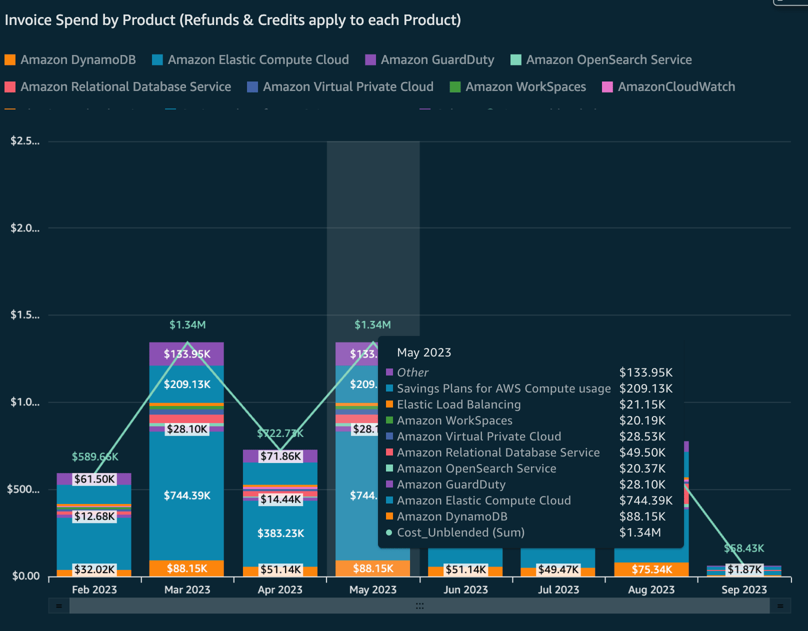
Figure: CUDOS Dashboard Showing Monthly Spend by Service.
Source: AWS Demo CUDOS Dashboard.

The six dashboards that comprise the set of Cloud Intelligence Dashboards are:

1. Cost Intelligence Dashboard (CID) – Meant to be “the foundation of your own cost management and optimization (FinOps) tool.” This dashboard is focused on looking at spend, chargeback, savings plan, reserved instances and other financial services on an account level. This is useful for understanding which accounts (and thus, business units) are driving AWS spend.
2. KPI Dashboard – The KPI dashboard tracks progress toward common goals. Not surprisingly, these goals are exactly what both AWS and we at CloudFix have been recommending: turning on S3 Intelligent-Tiering, using Graviton or AMD, moving your EBS volumes to gp3, etc. This dashboard shows progress towards these goals, such as the percentage of running instances that are using Graviton.
3. CUDOS Dashboard – As summarized above, the CUDOS dashboard provides the most comprehensive cost and usage details. Check out this blog post about using the CUDOS Dashboard, by Yuriy Prykhodko and Michael Herger. This dashboard and the Cloud Intelligence Dashboard are considered the foundational dashboards within the Cloud Intelligence Dashboards suite.
4. Data Transfer and Trends Dashboards – These two dashboards are relatively new and in development. They attempt to give insights into the amounts of data transfer (which can be a significant cost) and trends in usage, respectively.
5. Trusted Advisor Organizational (TAO) Dashboard – Trusted Advisor gives recommendations on security, cost optimization, fault tolerance, and more. Trusted Advisor also provides alerts regarding idle RDS instances and low utilization RDS instances.
6. Compute Optimizer Dashboard (COD) – AWS Compute Optimizer gives recommendations for right-sizing EC2 instances, Lambda, AutoScaling Groups, and EBS file systems. WIth the COD, we can track potential savings suggested by Compute Optimizer. We recently interviewed Rick Ochs, AWS Optimization Lead, about this dashboard. Check out the full episode here.

See the Getting Started with CUDOS, KPI, and Cost Intelligence Dashboards document for information on how to deploy these in your AWS account. Interestingly, all of these dashboards are based on AWS technologies, in particular the Cost and Usage Report, Athena, S3, and QuickSight to name a few. If you click on each of the links above, the Cloud Intelligence Dashboard team has put together demo dashboards that you can interact with, using sample data.

In our AWS Made Easy livestream, Rahul and I interviewed Yuriy Prykhodko, Principal TAM and Cloud Intelligence Dashboard Lead, and had an in-depth discussion on the Cloud Intelligence Dashboards. The full episode is available below, and on our AWS Made Easy YouTube channel.

6. Go forth and save!

Even with all that information, we’ve barely scratched the surface of what can be done with the AWS Cost and Usage report. It really is unbelievably powerful to have an hourly analysis and detailed data of every dollar spent in your organization. 

A few final thoughts and recommendations:

• Take the time to set up, learn, and use the Cost and Usage Report. Query it with Athena.
• You can find particular types of resources by matching on the distinctive ARNs, and also using the Product/Description field where applicable.
• Be sure to explore the relationships between the different fields, especially which LineItem/UsageType fields will appear for a particular combination of LineItem/LineItemType and resource type.

That’s a wrap on the CUR. Check back often for new Fixer and Foundation blogs: all part of our mission to help you spend less on AWS.